How to Read Training Set in Numpy
One of the key aspects of supervised automobile learning is model evaluation and validation. When you evaluate the predictive performance of your model, information technology's essential that the process exist unbiased. Using train_test_split() from the data science library scikit-acquire, you can split your dataset into subsets that minimize the potential for bias in your evaluation and validation process.
In this tutorial, y'all'll larn:
- Why you need to dissever your dataset in supervised machine learning
- Which subsets of the dataset you need for an unbiased evaluation of your model
- How to utilise
train_test_split()to dissever your data - How to combine
train_test_split()with prediction methods
In addition, y'all'll get information on related tools from sklearn.model_selection.
The Importance of Data Splitting
Supervised machine learning is virtually creating models that precisely map the given inputs (independent variables, or predictors) to the given outputs (dependent variables, or responses).
How yous measure the precision of your model depends on the type of a trouble you're trying to solve. In regression assay, you typically use the coefficient of decision, root-mean-square fault, mean absolute error, or similar quantities. For classification problems, you lot often apply accuracy, precision, recall, F1 score, and related indicators.
The acceptable numeric values that measure precision vary from field to field. Yous can notice detailed explanations from Statistics By Jim, Quora, and many other resources.
What'south nigh of import to understand is that you ordinarily need unbiased evaluation to properly use these measures, assess the predictive functioning of your model, and validate the model.
This means that you lot can't evaluate the predictive performance of a model with the same data you lot used for training. You need evaluate the model with fresh information that hasn't been seen by the model before. You can attain that past splitting your dataset before you utilise it.
Preparation, Validation, and Exam Sets
Splitting your dataset is essential for an unbiased evaluation of prediction performance. In most cases, it'south plenty to split your dataset randomly into 3 subsets:
-
The preparation set is applied to train, or fit, your model. For example, you use the training set to notice the optimal weights, or coefficients, for linear regression, logistic regression, or neural networks.
-
The validation set is used for unbiased model evaluation during hyperparameter tuning. For instance, when you want to find the optimal number of neurons in a neural network or the best kernel for a support vector auto, you experiment with different values. For each considered setting of hyperparameters, you fit the model with the training set and assess its performance with the validation set up.
-
The test fix is needed for an unbiased evaluation of the concluding model. You shouldn't utilize information technology for fitting or validation.
In less complex cases, when you don't have to tune hyperparameters, it's okay to work with but the training and test sets.
Underfitting and Overfitting
Splitting a dataset might also exist important for detecting if your model suffers from one of two very common issues, called underfitting and overfitting:
-
Underfitting is usually the consequence of a model being unable to encapsulate the relations among data. For example, this can happen when trying to correspond nonlinear relations with a linear model. Underfitted models volition probable take poor performance with both training and test sets.
-
Overfitting unremarkably takes place when a model has an excessively complex structure and learns both the existing relations among data and noise. Such models often take bad generalization capabilities. Although they work well with training data, they usually yield poor performance with unseen (exam) data.
You lot tin can find a more than detailed explanation of underfitting and overfitting in Linear Regression in Python.
Prerequisites for Using train_test_split()
At present that you understand the need to split a dataset in gild to perform unbiased model evaluation and place underfitting or overfitting, you're gear up to learn how to split your own datasets.
You'll utilize version 0.23.1 of scikit-larn, or sklearn . It has many packages for data science and machine learning, but for this tutorial you'll focus on the model_selection package, specifically on the office train_test_split() .
You can install sklearn with pip install:
$ python -m pip install -U "scikit-learn==0.23.1" If you employ Anaconda, then you probably already have information technology installed. Nevertheless, if you want to use a fresh surroundings, ensure that you take the specified version, or use Miniconda, so yous can install sklearn from Anaconda Cloud with conda install:
$ conda install -c anaconda scikit-learn= 0.23 You lot'll too need NumPy, but you don't take to install it separately. Y'all should become it forth with sklearn if you don't already accept it installed. If yous want to refresh your NumPy noesis, then accept a look at the official documentation or check out Look Ma, No For-Loops: Array Programming With NumPy.
Application of train_test_split()
You need to import train_test_split() and NumPy before you can employ them, so y'all tin start with the import statements:
>>>
>>> import numpy as np >>> from sklearn.model_selection import train_test_split Now that y'all have both imported, you can utilise them to dissever information into preparation sets and test sets. You'll split inputs and outputs at the same time, with a single part call.
With train_test_split(), you need to provide the sequences that you want to separate every bit well as any optional arguments. It returns a list of NumPy arrays, other sequences, or SciPy thin matrices if appropriate:
sklearn . model_selection . train_test_split ( * arrays , ** options ) -> listing arrays is the sequence of lists, NumPy arrays, pandas DataFrames, or similar array-similar objects that hold the information you want to separate. All these objects together brand upward the dataset and must be of the same length.
In supervised machine learning applications, you'll typically work with two such sequences:
- A ii-dimensional array with the inputs (
ten) - A one-dimensional array with the outputs (
y)
options are the optional keyword arguments that you can employ to become desired behavior:
-
train_sizeis the number that defines the size of the training prepare. If you provide afloat, and so it must be betwixt0.0andane.0and will define the share of the dataset used for testing. If you provide anint, then information technology volition correspond the total number of the training samples. The default value isNone. -
test_sizeis the number that defines the size of the exam gear up. It'due south very similar totrain_size. Yous should provide eithertrain_sizeortest_size. If neither is given, and then the default share of the dataset that will be used for testing is0.25, or 25 pct. -
random_stateis the object that controls randomization during splitting. It can exist either anintor an instance ofRandomState. The default value isNone. -
shuffleis the Boolean object (Trueby default) that determines whether to shuffle the dataset before applying the split. -
stratifyis an array-like object that, if nonNone, determines how to use a stratified split.
Now it's fourth dimension to attempt data splitting! You'll start by creating a simple dataset to piece of work with. The dataset will contain the inputs in the two-dimensional array 10 and outputs in the i-dimensional array y:
>>>
>>> x = np . arange ( one , 25 ) . reshape ( 12 , 2 ) >>> y = np . array ([ 0 , i , one , 0 , 1 , 0 , 0 , 1 , 1 , 0 , 1 , 0 ]) >>> x array([[ i, 2], [ three, iv], [ 5, 6], [ 7, 8], [ 9, x], [11, 12], [13, 14], [xv, sixteen], [17, 18], [19, xx], [21, 22], [23, 24]]) >>> y array([0, ane, 1, 0, 1, 0, 0, ane, i, 0, 1, 0]) To get your data, you use arange(), which is very convenient for generating arrays based on numerical ranges. You besides use .reshape() to alter the shape of the assortment returned past arange() and get a 2-dimensional data structure.
Yous tin dissever both input and output datasets with a unmarried function call:
>>>
>>> x_train , x_test , y_train , y_test = train_test_split ( x , y ) >>> x_train array([[15, 16], [21, 22], [11, 12], [17, 18], [13, 14], [ nine, 10], [ 1, ii], [ three, 4], [19, twenty]]) >>> x_test array([[ 5, half dozen], [ 7, viii], [23, 24]]) >>> y_train array([1, 1, 0, 1, 0, 1, 0, 1, 0]) >>> y_test array([1, 0, 0]) Given two sequences, like x and y here, train_test_split() performs the split and returns 4 sequences (in this example NumPy arrays) in this order:
-
x_train: The training part of the first sequence (x) -
x_test: The test part of the offset sequence (x) -
y_train: The grooming part of the 2nd sequence (y) -
y_test: The test part of the second sequence (y)
You probably got different results from what you run into here. This is considering dataset splitting is random by default. The result differs each fourth dimension you run the function. Still, this often isn't what you want.
Sometimes, to brand your tests reproducible, you demand a random split with the same output for each office telephone call. You lot can do that with the parameter random_state. The value of random_state isn't important—it can exist any non-negative integer. You could utilise an case of numpy.random.RandomState instead, only that is a more than complex approach.
In the previous example, yous used a dataset with twelve observations (rows) and got a training sample with ix rows and a exam sample with three rows. That's because you didn't specify the desired size of the training and examination sets. By default, 25 pct of samples are assigned to the test ready. This ratio is by and large fine for many applications, but it'south not e'er what you demand.
Typically, you lot'll want to define the size of the examination (or preparation) fix explicitly, and sometimes you'll fifty-fifty desire to experiment with unlike values. You can practise that with the parameters train_size or test_size.
Modify the code so you lot tin choose the size of the examination set up and become a reproducible result:
>>>
>>> x_train , x_test , y_train , y_test = train_test_split ( ... x , y , test_size = 4 , random_state = 4 ... ) >>> x_train array([[17, 18], [ 5, 6], [23, 24], [ i, two], [ 3, iv], [11, 12], [15, 16], [21, 22]]) >>> x_test array([[ 7, 8], [ 9, 10], [thirteen, 14], [19, twenty]]) >>> y_train array([one, 1, 0, 0, one, 0, 1, 1]) >>> y_test assortment([0, 1, 0, 0]) With this change, y'all get a different result from before. Earlier, you had a training set with 9 items and test set with three items. Now, thanks to the argument test_size=4, the training set has eight items and the test set has four items. You'd get the aforementioned result with test_size=0.33 because 33 percent of twelve is approximately iv.
There's one more very important difference between the last 2 examples: Yous now become the same consequence each time you run the function. This is because you've fixed the random number generator with random_state=4.
The figure below shows what's going on when you call train_test_split():
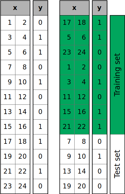
The samples of the dataset are shuffled randomly and then split into the training and test sets according to the size you defined.
You can see that y has vi zeros and vi ones. However, the test set has iii zeros out of 4 items. If you want to (approximately) proceed the proportion of y values through the grooming and test sets, and so pass stratify=y. This will enable stratified splitting:
>>>
>>> x_train , x_test , y_train , y_test = train_test_split ( ... x , y , test_size = 0.33 , random_state = 4 , stratify = y ... ) >>> x_train array([[21, 22], [ 1, 2], [15, sixteen], [13, fourteen], [17, 18], [19, twenty], [23, 24], [ three, 4]]) >>> x_test array([[11, 12], [ 7, viii], [ 5, six], [ 9, 10]]) >>> y_train assortment([1, 0, 1, 0, 1, 0, 0, ane]) >>> y_test assortment([0, 0, 1, ane]) Now y_train and y_test accept the aforementioned ratio of zeros and ones as the original y array.
Stratified splits are desirable in some cases, like when y'all're classifying an imbalanced dataset, a dataset with a pregnant difference in the number of samples that belong to distinct classes.
Finally, you tin turn off data shuffling and random split with shuffle=Simulated:
>>>
>>> x_train , x_test , y_train , y_test = train_test_split ( ... ten , y , test_size = 0.33 , shuffle = False ... ) >>> x_train assortment([[ i, two], [ 3, 4], [ five, six], [ 7, viii], [ 9, 10], [11, 12], [13, 14], [xv, 16]]) >>> x_test assortment([[17, 18], [19, twenty], [21, 22], [23, 24]]) >>> y_train array([0, 1, i, 0, i, 0, 0, 1]) >>> y_test array([one, 0, i, 0]) Now you have a split in which the first ii-thirds of samples in the original 10 and y arrays are assigned to the training set and the last third to the test set. No shuffling. No randomness.
Supervised Machine Learning With train_test_split()
Now information technology's time to see train_test_split() in action when solving supervised learning problems. Y'all'll start with a minor regression problem that can exist solved with linear regression before looking at a bigger problem. Y'all'll also come across that you can use train_test_split() for classification as well.
Minimalist Example of Linear Regression
In this instance, y'all'll apply what you've learned then far to solve a modest regression problem. You lot'll learn how to create datasets, split them into training and test subsets, and utilize them for linear regression.
As always, you lot'll outset by importing the necessary packages, functions, or classes. You'll need NumPy, LinearRegression, and train_test_split():
>>>
>>> import numpy equally np >>> from sklearn.linear_model import LinearRegression >>> from sklearn.model_selection import train_test_split Now that y'all've imported everything you demand, you can create two pocket-sized arrays, 10 and y, to stand for the observations and and so split them into training and examination sets just as you did before:
>>>
>>> x = np . arange ( twenty ) . reshape ( - ane , 1 ) >>> y = np . array ([ 5 , 12 , 11 , nineteen , 30 , 29 , 23 , 40 , 51 , 54 , 74 , ... 62 , 68 , 73 , 89 , 84 , 89 , 101 , 99 , 106 ]) >>> x array([[ 0], [ 1], [ two], [ 3], [ 4], [ v], [ 6], [ seven], [ 8], [ 9], [10], [xi], [12], [thirteen], [14], [xv], [16], [17], [18], [19]]) >>> y array([ 5, 12, 11, 19, xxx, 29, 23, 40, 51, 54, 74, 62, 68, 73, 89, 84, 89, 101, 99, 106]) >>> x_train , x_test , y_train , y_test = train_test_split ( ... x , y , test_size = 8 , random_state = 0 ... ) Your dataset has twenty observations, or x-y pairs. You specify the argument test_size=eight, then the dataset is divided into a training set with twelve observations and a examination gear up with eight observations.
At present y'all can use the training set to fit the model:
>>>
>>> model = LinearRegression () . fit ( x_train , y_train ) >>> model . intercept_ 3.1617195496417523 >>> model . coef_ assortment([5.53121801]) LinearRegression creates the object that represents the model, while .fit() trains, or fits, the model and returns information technology. With linear regression, fitting the model means determining the best intercept (model.intercept_) and gradient (model.coef_) values of the regression line.
Although you can use x_train and y_train to bank check the goodness of fit, this isn't a all-time exercise. An unbiased estimation of the predictive performance of your model is based on exam data:
>>>
>>> model . score ( x_train , y_train ) 0.9868175024574795 >>> model . score ( x_test , y_test ) 0.9465896927715023 .score() returns the coefficient of determination, or R², for the data passed. Its maximum is 1. The higher the R² value, the better the fit. In this example, the preparation data yields a slightly higher coefficient. Nonetheless, the R² calculated with examination data is an unbiased measure of your model'southward prediction performance.
This is how it looks on a graph:
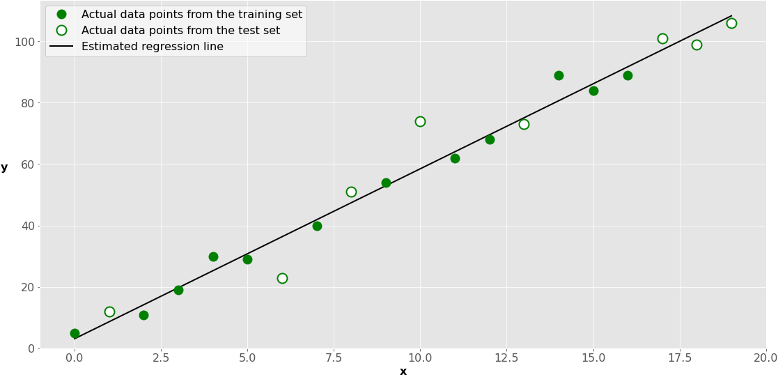
The green dots represent the 10-y pairs used for training. The black line, called the estimated regression line, is defined by the results of model fitting: the intercept and the gradient. So, it reflects the positions of the dark-green dots only.
The white dots represent the test set. Y'all use them to estimate the performance of the model (regression line) with data not used for training.
Regression Example
Now you're ready to split a larger dataset to solve a regression problem. You'll use a well-known Boston firm prices dataset, which is included in sklearn. This dataset has 506 samples, xiii input variables, and the house values equally the output. You can retrieve it with load_boston().
First, import train_test_split() and load_boston():
>>>
>>> from sklearn.datasets import load_boston >>> from sklearn.model_selection import train_test_split Now that you take both functions imported, yous tin get the data to work with:
>>>
>>> ten , y = load_boston ( return_X_y = Truthful ) Equally yous tin see, load_boston() with the argument return_X_y=True returns a tuple with two NumPy arrays:
- A two-dimensional array with the inputs
- A one-dimensional array with the outputs
The next stride is to separate the data the same way as before:
>>>
>>> x_train , x_test , y_train , y_test = train_test_split ( ... x , y , test_size = 0.4 , random_state = 0 ... ) At present y'all have the training and test sets. The grooming information is contained in x_train and y_train, while the data for testing is in x_test and y_test.
When you work with larger datasets, it's usually more convenient to laissez passer the grooming or test size as a ratio. test_size=0.four ways that approximately forty percent of samples volition be assigned to the exam data, and the remaining threescore percent will be assigned to the training data.
Finally, you tin use the training set (x_train and y_train) to fit the model and the test fix (x_test and y_test) for an unbiased evaluation of the model. In this example, yous'll apply three well-known regression algorithms to create models that fit your data:
- Linear regression with
LinearRegression() - Slope boosting with
GradientBoostingRegressor() - Random forest with
RandomForestRegressor()
The process is pretty much the aforementioned as with the previous example:
- Import the classes you need.
- Create model instances using these classes.
- Fit the model instances with
.fit()using the training gear up. - Evaluate the model with
.score()using the test set.
Here's the lawmaking that follows the steps described above for all three regression algorithms:
>>>
>>> from sklearn.linear_model import LinearRegression >>> model = LinearRegression () . fit ( x_train , y_train ) >>> model . score ( x_train , y_train ) 0.7668160223286261 >>> model . score ( x_test , y_test ) 0.6882607142538016 >>> from sklearn.ensemble import GradientBoostingRegressor >>> model = GradientBoostingRegressor ( random_state = 0 ) . fit ( x_train , y_train ) >>> model . score ( x_train , y_train ) 0.9859065238883613 >>> model . score ( x_test , y_test ) 0.8530127436482149 >>> from sklearn.ensemble import RandomForestRegressor >>> model = RandomForestRegressor ( random_state = 0 ) . fit ( x_train , y_train ) >>> model . score ( x_train , y_train ) 0.9811695664860354 >>> model . score ( x_test , y_test ) 0.8325867908704008 You've used your training and examination datasets to fit 3 models and evaluate their performance. The measure of accuracy obtained with .score() is the coefficient of conclusion. It tin be calculated with either the preparation or test set. Withal, equally you lot already learned, the score obtained with the exam gear up represents an unbiased estimation of performance.
Equally mentioned in the documentation, you can provide optional arguments to LinearRegression(), GradientBoostingRegressor(), and RandomForestRegressor(). GradientBoostingRegressor() and RandomForestRegressor() use the random_state parameter for the same reason that train_test_split() does: to deal with randomness in the algorithms and ensure reproducibility.
For some methods, you lot may also need feature scaling. In such cases, yous should fit the scalers with training data and utilise them to transform test information.
Classification Example
You can use train_test_split() to solve classification bug the aforementioned way you do for regression analysis. In machine learning, classification bug involve grooming a model to utilize labels to, or classify, the input values and sort your dataset into categories.
In the tutorial Logistic Regression in Python, you'll find an case of a handwriting recognition job. The example provides another demonstration of splitting data into training and test sets to avoid bias in the evaluation procedure.
Other Validation Functionalities
The bundle sklearn.model_selection offers a lot of functionalities related to model selection and validation, including the following:
- Cross-validation
- Learning curves
- Hyperparameter tuning
Cantankerous-validation is a prepare of techniques that combine the measures of prediction performance to go more accurate model estimations.
1 of the widely used cross-validation methods is k-fold cross-validation. In it, y'all split up your dataset into g (frequently five or 10) subsets, or folds, of equal size and so perform the preparation and test procedures 1000 times. Each time, y'all use a different fold as the test set and all the remaining folds as the training set. This provides thousand measures of predictive performance, and you lot can then clarify their hateful and standard deviation.
You can implement cross-validation with KFold, StratifiedKFold, LeaveOneOut, and a few other classes and functions from sklearn.model_selection.
A learning curve, sometimes called a preparation curve, shows how the prediction score of training and validation sets depends on the number of training samples. You can use learning_curve() to become this dependency, which tin assist you lot find the optimal size of the preparation set, cull hyperparameters, compare models, and and then on.
Hyperparameter tuning, also called hyperparameter optimization, is the process of determining the all-time set of hyperparameters to define your machine learning model. sklearn.model_selection provides you with several options for this purpose, including GridSearchCV, RandomizedSearchCV, validation_curve(), and others. Splitting your data is also important for hyperparameter tuning.
Decision
Yous now know why and how to use train_test_split() from sklearn. Yous've learned that, for an unbiased interpretation of the predictive performance of car learning models, you should employ data that hasn't been used for model plumbing equipment. That's why you demand to split your dataset into training, test, and in some cases, validation subsets.
In this tutorial, you've learned how to:
- Use
train_test_split()to get grooming and test sets - Control the size of the subsets with the parameters
train_sizeandtest_size - Make up one's mind the randomness of your splits with the
random_stateparameter - Obtain stratified splits with the
stratifyparameter - Utilise
train_test_split()as a part of supervised machine learning procedures
You lot've besides seen that the sklearn.model_selection module offers several other tools for model validation, including cross-validation, learning curves, and hyperparameter tuning.
If y'all have questions or comments, then please put them in the comment department below.
Source: https://realpython.com/train-test-split-python-data/
0 Response to "How to Read Training Set in Numpy"
Post a Comment